Postprocessing on isoscan

Example of isoscan postprocessing procedures. The data are a deflector scan on graphene as simulated from a third nearest neighbor tight binding model. The same workflow can be applied to any tilt-, polar-, deflector- or hv-scan.

Import the “fundamental” python libraries for a generic data analysis:

import numpy as np

Instead of loading the file as for example:

# from navarp.utils import navfile
# file_name = r"nxarpes_simulated_cone.nxs"
# entry = navfile.load(file_name)

Here we build the simulated graphene signal with a dedicated function defined just for this purpose:

from navarp.extras.simulation import get_tbgraphene_deflector

entry = get_tbgraphene_deflector(
    scans=np.linspace(-0.1, 0.1, 3),
    angles=np.linspace(-25, 6, 400),
    ebins=np.linspace(-13, 0.4, 700),
    tht_an=-18,
    phi_an=0,
    hv=120,
    gamma=0.05
)

Fermi level autoset

entry.autoset_efermi(scan_range=[-2, 2], energy_range=[115.2, 115.8])
print("Energy of the Fermi level = {:.0f} eV".format(entry.efermi))
print("Energy resolution = {:.0f} meV".format(entry.efermi_fwhm*1000))

entry.plt_efermi_fit()

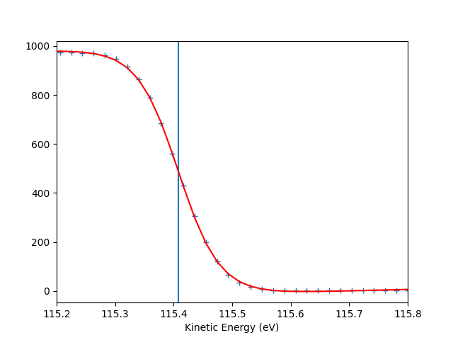
Fermi level at 115.4081 eV
Energy resolution = 140.2 meV (i.e. FWHM of the Gaussian shape which, convoluted with a step function, fits the Fermi edge)
Photon energy is now set to 120.0081 eV (instead of 120.0000 eV)
Energy of the Fermi level = 115 eV
Energy resolution = 140 meV

Set the k-space for the transformation

entry.set_kspace(
    tht_p=0.1,
    k_along_slit_p=1.7,
    scan_p=0,
    ks_p=0,
    e_kin_p=114.3,
)

tht_an = -17.979
scan_type =  deflector
inn_pot = 14.000
scans_0 = 0.000
phi_an = 0.000
kspace transformation ready

Post processing on the isoscan:

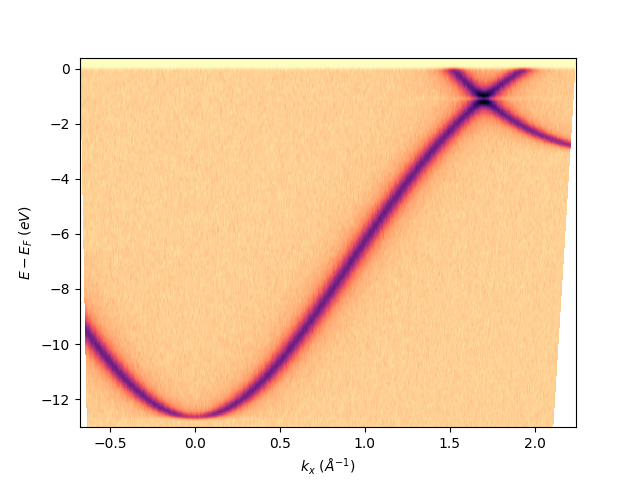
First of all let’s show it:

entry.isoscan(0).show()

<matplotlib.collections.QuadMesh object at 0x78b8eaad8f70>

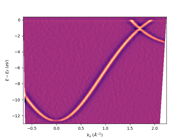
The second derivative can be obtained using sigma in the definition, which define the extension in points of the Gaussian filter used to then get the second derivative. In this case the sigma is different from zero only on the second element, meaning that the derivative will be performed only along the energy axis: sphinx_gallery_thumbnail_number = 3

entry.isoscan(0, sigma=[3, 5]).show()

<matplotlib.collections.QuadMesh object at 0x78b8ea8f6bc0>

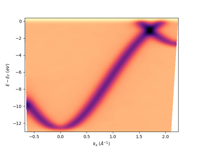
Only the Gaussian filtered image can be obtained using again sigma but also specifying the order=0, which by default is equal to 2 giving the second derivative as before.:

entry.isoscan(0, sigma=[10, 10], order=0).show()

<matplotlib.collections.QuadMesh object at 0x78b8ea8c5b40>

To export it as NXdata class of the nexus format uncomment this line:

# entry.isoscan(0, 0, sigma=[3, 5], order=0).export_as_nxs('fermimap.nxs')

To export it as igor-pro text file (itx) uncomment this line:

# entry.isoscan(0, 0, sigma=[3, 5], order=0).export_as_itx('fermimap.itx')