Export isoenergy at the Fermi level

Simple workflow for exporting the isoenergy at the Fermi level. The data are a deflector scan on graphene as simulated from a third nearest neighbor tight binding model. The same workflow can be applied to any tilt-, polar-, deflector- or hv-scan.

Import the “fundamental” python libraries for a generic data analysis:

import numpy as np

Instead of loading the file as for example:

# from navarp.utils import navfile
# file_name = r"nxarpes_simulated_cone.nxs"
# entry = navfile.load(file_name)

Here we build the simulated graphene signal with a dedicated function defined just for this purpose:

from navarp.extras.simulation import get_tbgraphene_deflector

entry = get_tbgraphene_deflector(
    scans=np.linspace(-5., 20., 91),
    angles=np.linspace(-25, 6, 400),
    ebins=np.linspace(-13, 0.4, 700),
    tht_an=-18,
    phi_an=0,
    hv=120,
    gamma=0.05
)

Fermi level autoset

entry.autoset_efermi(scan_range=[-5, 5], energy_range=[115.2, 115.8])
print("Energy of the Fermi level = {:.0f} eV".format(entry.efermi))
print("Energy resolution = {:.0f} meV".format(entry.efermi_fwhm*1000))

entry.plt_efermi_fit()

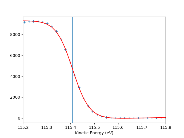
Fermi level at 115.4094 eV
Energy resolution = 137.8 meV (i.e. FWHM of the Gaussian shape which, convoluted with a step function, fits the Fermi edge)
Photon energy is now set to 120.0094 eV (instead of 120.0000 eV)
Energy of the Fermi level = 115 eV
Energy resolution = 138 meV

Set the k-space for the transformation

entry.set_kspace(
    tht_p=0.1,
    k_along_slit_p=1.7,
    scan_p=0,
    ks_p=0,
    e_kin_p=114.3,
)

tht_an = -17.979
scan_type =  deflector
inn_pot = 14.000
scans_0 = 0.000
phi_an = 0.000
kspace transformation ready

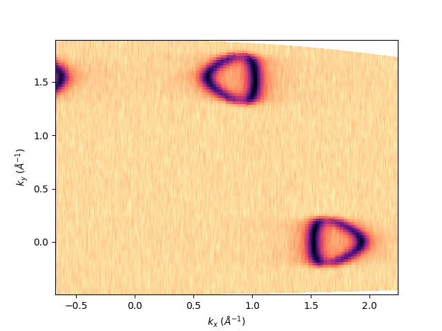
Export the Fermi surface:

First of all let’s show it:

entry.isoenergy(0, 0.02).show()

<matplotlib.collections.QuadMesh object at 0x7f6262841690>

Then to be exported it mush be interpolated in a uniform grid. This can be done by defining kbins in the isoenergy definition, which is the number of points the momentum along the analyzer slit and the scan. In this case the number will be [1000, 800] and we will call such isoenergy object as isoatfermi. sphinx_gallery_thumbnail_number = 3

isoatfermi = entry.isoenergy(0, 0.02, kbins=[1000, 800])

To show what we are going to save, the method is always the same:

isoatfermi.show()

<matplotlib.collections.QuadMesh object at 0x7f6262bb33a0>

To export it as NXdata class of the nexus format uncomment this line:

# isoatfermi.export_as_nxs('fermimap.nxs')

To export it as igor-pro text file (itx) uncomment this line:

# isoatfermi.export_as_itx('fermimap.itx')