Interpolation on Graphene deflector scan

Simple workflow for the interpolation of data along a generic path in the k-space from its isoenergy cuts. The data are a deflector scan on graphene as simulated from a third nearest neighbor tight binding model. The same workflow can be applied to any tilt-, polar-, deflector- or hv-scan.

Import the “fundamental” python libraries for a generic data analysis:

import numpy as np
import matplotlib.pyplot as plt

Instead of loading the file as for example:

# from navarp.utils import navfile
# file_name = r"nxarpes_simulated_cone.nxs"
# entry = navfile.load(file_name)

Here we build the simulated graphene signal with a dedicated function defined just for this purpose:

from navarp.extras.simulation import get_tbgraphene_deflector

entry = get_tbgraphene_deflector(
    scans=np.linspace(-5., 20., 91),
    angles=np.linspace(-25, 6, 400),
    ebins=np.linspace(-13, 0.4, 700),
    tht_an=-18,
    phi_an=0,
    hv=120,
    gamma=0.05
)

Fermi level autoset

entry.autoset_efermi(scan_range=[-5, 5], energy_range=[115.2, 115.8])
print("Energy of the Fermi level = {:.0f} eV".format(entry.efermi))
print("Energy resolution = {:.0f} meV".format(entry.efermi_fwhm*1000))

entry.plt_efermi_fit()

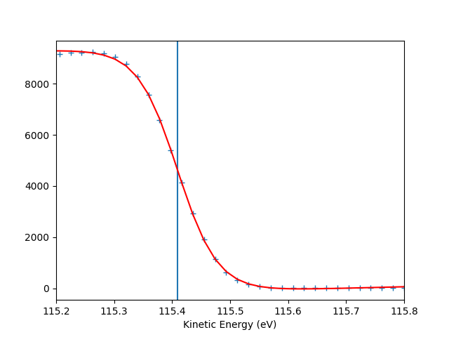
Fermi level at 115.4093 eV
Energy resolution = 137.8 meV (i.e. FWHM of the Gaussian shape which, convoluted with a step function, fits the Fermi edge)
Photon energy is now set to 120.0093 eV (instead of 120.0000 eV)
Energy of the Fermi level = 115 eV
Energy resolution = 138 meV

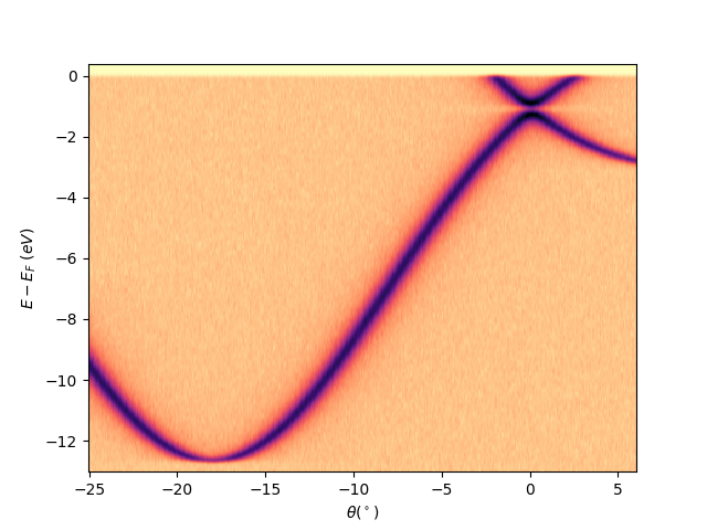
Check for the Fermi level alignment

entry.isoscan(scan=0, dscan=0).show(yname='eef')

<matplotlib.collections.QuadMesh object at 0x7f626272d420>

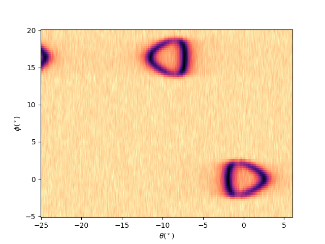
Plotting iso-energetic cut at ekin = efermi

entry.isoenergy(0, 0.02).show()

<matplotlib.collections.QuadMesh object at 0x7f6262bfe6e0>

Set the k-space for the transformation

entry.set_kspace(
    tht_p=0.1,
    k_along_slit_p=1.7,
    scan_p=0,
    ks_p=0,
    e_kin_p=114.3,
)

tht_an = -17.979
scan_type =  deflector
inn_pot = 14.000
scans_0 = 0.000
phi_an = 0.000
kspace transformation ready

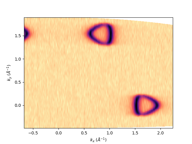
and check the isoenergy at the Fermi level:

entry.isoenergy(0, 0.02).show()

<matplotlib.collections.QuadMesh object at 0x7f62628dec50>

Define the interpolation path points

kbins = 900
k_GK = 1.702
k_pts_xy = np.array([
    [0, 0],
    [k_GK, 0],
    [k_GK*np.cos(np.pi/3), k_GK*np.sin(np.pi/3)+0.05],
    [0, 0]
])
kx_pts = k_pts_xy[:, 0]
ky_pts = k_pts_xy[:, 1]

klabels = [
    r'$\Gamma$',
    r'$\mathrm{K}$',
    r'$\mathrm{K}^{\prime}$',
    r'$\Gamma$'
]

and show them on the isoenergy at the Dirac point energy:

entry.isoenergy(-1.1, 0.02).show()
plt.plot(kx_pts, ky_pts, '-+')

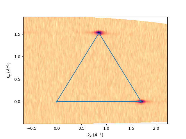
[<matplotlib.lines.Line2D object at 0x7f6262785d80>]

Run the interpolation defining an isok:

isok = entry.isok(kx_pts, ky_pts, klabels)

Show the final results with the executed path on the isoenergy: sphinx_gallery_thumbnail_number = 6

fig, axs = plt.subplots(1, 2)

entry.isoenergy(0, 0.02).show(ax=axs[0])

isok.path_show(axs[0], 'k', 'k', xytext=(8, 8))

qmesh = isok.show(ax=axs[1])

fig.tight_layout()
fig.colorbar(qmesh)

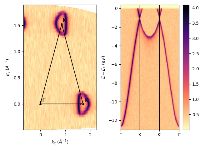
<matplotlib.colorbar.Colorbar object at 0x7f62627dd030>