Graphene deflector scan

Simple workflow for analyzing a deflector scan data of graphene as simulated from a third nearest neighbor tight binding model. The same workflow can be applied to any tilt-, polar- or deflector-scan.

Import the “fundamental” python libraries for a generic data analysis:

import numpy as np
import matplotlib.pyplot as plt

Instead of loading the file as for example:

# from navarp.utils import navfile
# file_name = r"nxarpes_simulated_cone.nxs"
# entry = navfile.load(file_name)

Here we build the simulated graphene signal with a dedicated function defined just for this purpose:

from navarp.extras.simulation import get_tbgraphene_deflector

entry = get_tbgraphene_deflector(
    scans=np.linspace(-5., 5., 51),
    angles=np.linspace(-7, 7, 300),
    ebins=np.linspace(-3.3, 0.4, 450),
    tht_an=-18,
    phi_an=0,
    hv=120
)

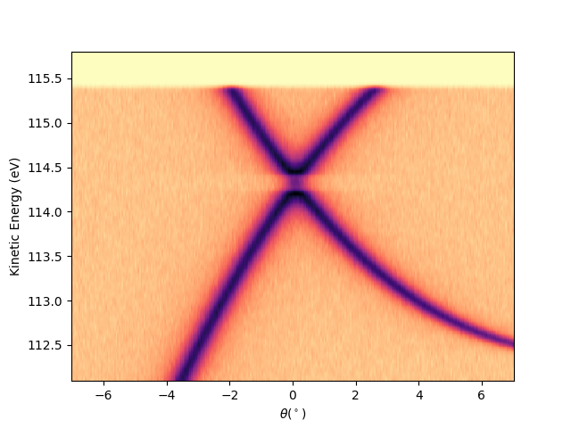
Plot a single analyzer image at scan = 0

First I have to extract the isoscan from the entry, so I use the isoscan method of entry:

iso0 = entry.isoscan(scan=0, dscan=0)

Then to plot it using the ‘show’ method of the extracted iso0:

iso0.show(yname='ekin')

<matplotlib.collections.QuadMesh object at 0x7f62627dc190>

Or by string concatenation, directly as:

entry.isoscan(scan=0, dscan=0).show(yname='ekin')

<matplotlib.collections.QuadMesh object at 0x7f6262211930>

Fermi level determination

The initial guess for the binding energy is: ebins = ekins - (hv - work_fun). However, the better way is to proper set the Fermi level first and then derives everything form it. The Fermi level can be given directly as a value using:

entry.set_efermi(114.8)

Or it can be detected from a fit using the method autoset_efermi. In both cases the binding energy and the photon energy will be updated consistently. Note that the work function depends on the beamline or laboratory. If not specified is 4.5 eV.

entry.autoset_efermi(scan_range=[-5, 5], energy_range=[115.2, 115.8])
print("Energy of the Fermi level = {:.0f} eV".format(entry.efermi))
print("Energy resolution = {:.0f} meV".format(entry.efermi_fwhm*1000))

entry.plt_efermi_fit()

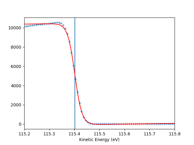
Fermi level at 115.4016 eV
Energy resolution = 56.5 meV (i.e. FWHM of the Gaussian shape which, convoluted with a step function, fits the Fermi edge)
Photon energy is now set to 120.0016 eV (instead of 120.0000 eV)
Energy of the Fermi level = 115 eV
Energy resolution = 57 meV

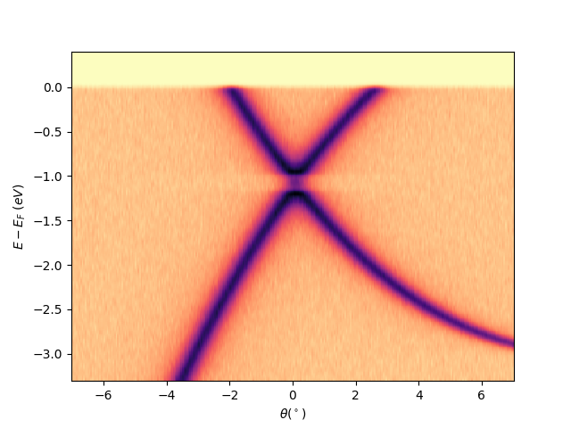
Plot a single analyzer image at scan = 0 with the Fermi level aligned

entry.isoscan(scan=0, dscan=0).show(yname='eef')

<matplotlib.collections.QuadMesh object at 0x7f6262293e80>

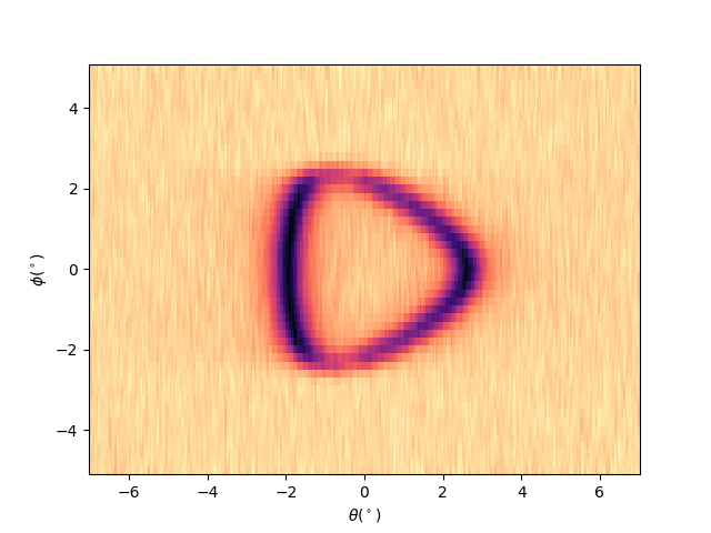
Plotting iso-energetic cut at ekin = efermi

entry.isoenergy(0).show()

<matplotlib.collections.QuadMesh object at 0x7f6262426680>

Plotting in the reciprocal space (k-space)

I have to define first the reference point to be used for the transformation. Meaning a point in the angular space which I know it correspond to a particular point in the k-space. In this case the graphene Dirac-point which is at ekin = 114.3 eV, in angle is at (tht_p, phi_p) = (0.1, 0) and in the k-space has to correspond to (kx, ky) = (1.7, 0).

entry.set_kspace(
    tht_p=0.1,
    k_along_slit_p=1.7,
    scan_p=0,
    ks_p=0,
    e_kin_p=114.3,
)

tht_an = -17.979
scan_type =  deflector
inn_pot = 14.000
scans_0 = 0.000
phi_an = 0.000
kspace transformation ready

Once it is set, all the isoscan or isoenergy extracted from the entry will now get their proper k-space scales:

entry.isoscan(0).show()

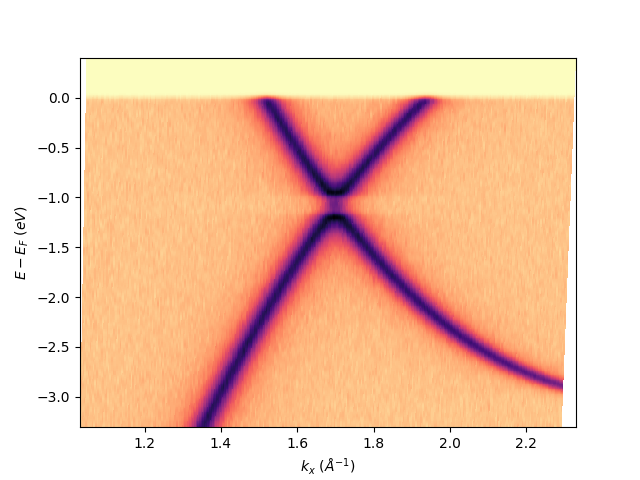
<matplotlib.collections.QuadMesh object at 0x7f6262479120>

# sphinx_gallery_thumbnail_number = 7

entry.isoenergy(0).show()

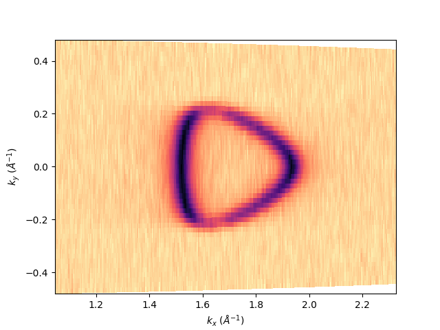
<matplotlib.collections.QuadMesh object at 0x7f62625ee8f0>

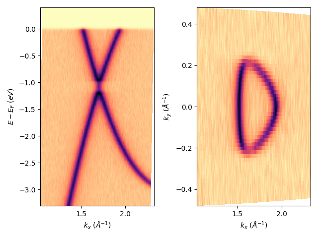
I can also place together in a single figure different images:

fig, axs = plt.subplots(1, 2)

entry.isoscan(0).show(ax=axs[0])
entry.isoenergy(0).show(ax=axs[1])

plt.tight_layout()

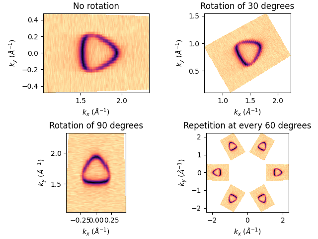
For the isoenergy case, I can also rotate the image around its origin. Which can be useful sometime if the sample was not exactly aligned during the data acquisition. Or if you are a fun on what I consider as a very bad practice, you can repeat the same image at each symmetric point.

fig, axs = plt.subplots(2, 2, constrained_layout=True)

ax = axs[0][0]
entry.isoenergy(0).show(ax=ax)
ax.set_title('No rotation'.format())

rot_ang = 30
ax = axs[0][1]
ax.set_title('Rotation of {} degrees'.format(rot_ang))
entry.isoenergy(0).show(ax=ax, rotate=rot_ang)

rot_ang = 90
ax = axs[1][0]
ax.set_title('Rotation of {} degrees'.format(rot_ang))
entry.isoenergy(0).show(ax=ax, rotate=rot_ang)

rot_angs = [0, 60, 120, 180, 240, 300]
ax = axs[1][1]
ax.set_title('Repetition at every 60 degrees')
isoen_fs = entry.isoenergy(0)
for rot_ang in rot_angs:
    isoen_fs.show(ax=ax, rotate=rot_ang)

for ax in axs.ravel():
    ax.set_aspect('equal')

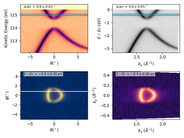
Many other options:

fig, axs = plt.subplots(2, 2)

scan = 0.8
dscan = 0.05
ebin = -0.4
debin = 0.05

entry.isoscan(scan, dscan).show(ax=axs[0][0], xname='tht', yname='ekin')
entry.isoscan(scan, dscan).show(ax=axs[0][1], cmap='binary')

axs[0][0].axhline(ebin-debin+entry.efermi)
axs[0][0].axhline(ebin+debin+entry.efermi)

axs[0][1].axhline(ebin-debin)
axs[0][1].axhline(ebin+debin)

entry.isoenergy(ebin, debin).show(
    ax=axs[1][0], xname='tht', yname='phi', cmap='cividis')
entry.isoenergy(ebin, debin).show(
    ax=axs[1][1], cmap='magma', cmapscale='log')

axs[1][0].axhline(scan, color='w')

x_note = 0.05
y_note = 0.98

for ax in axs[0][:]:
    ax.annotate(
        "$scan \: = \: {} \pm {} \; ^\circ$".format(scan, dscan),
        (x_note, y_note),
        xycoords='axes fraction',
        size=8, rotation=0, ha="left", va="top",
        bbox=dict(
            boxstyle="round", fc='w', alpha=0.65, edgecolor='None', pad=0.05
        )
    )

for ax in axs[1][:]:
    ax.annotate(
        "$E-E_F \: = \: {} \pm {} \; eV$".format(ebin, debin),
        (x_note, y_note),
        xycoords='axes fraction',
        size=8, rotation=0, ha="left", va="top",
        bbox=dict(
            boxstyle="round", fc='w', alpha=0.65, edgecolor='None', pad=0.05
        )
    )

plt.tight_layout()