Simulated cone basic analysis

Simple workflow for analyzing a deflector scan data. The same workflow can be applied in the case of manipulator angular scans.

Import the “fundamental” python libraries for a generic data analysis:

import numpy as np

Import the navarp libraries:

from navarp.utils import navfile

Load the data from a file:

file_name = r"nxarpes_simulated_cone.nxs"
entry = navfile.load(file_name)

instrument_name = simulated

Plot a single slice Ex: scan = 0.5

scan = 0.5
entry.isoscan(scan).show()

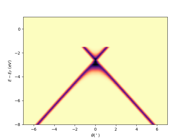
<matplotlib.collections.QuadMesh object at 0x7f62636627d0>

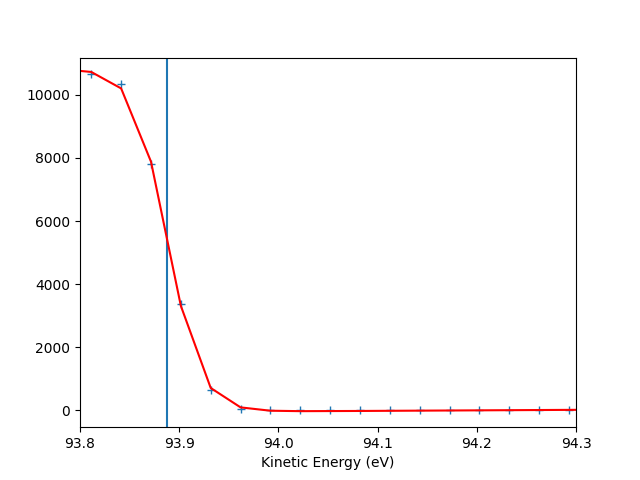
Fermi level determination

entry.autoset_efermi(energy_range=[93.8, 94.3])
entry.plt_efermi_fit()

print("Fermi level = {:.3f} meV".format(entry.efermi))
print("Energy resolution = {:.0f} meV".format(entry.efermi_fwhm*1000))
print("hv = {:g} eV".format(np.squeeze(entry.hv)))

/usr/local/lib/python3.10/site-packages/navarp/utils/fermilevel.py:67: RuntimeWarning: divide by zero encountered in divide
  ddata_s_denergies = ddata_s_denergies/np.abs(data_sum)
/usr/local/lib/python3.10/site-packages/navarp/utils/fermilevel.py:67: RuntimeWarning: invalid value encountered in divide
  ddata_s_denergies = ddata_s_denergies/np.abs(data_sum)
Fermi level at 93.8881 eV
Energy resolution = 67.2 meV (i.e. FWHM of the Gaussian shape which, convoluted with a step function, fits the Fermi edge)
Photon energy is now set to 98.4881 eV (instead of 100.0000 eV)
Fermi level = 93.888 meV
Energy resolution = 67 meV
hv = 98.4881 eV

Since now the Fermi level is known, the same plot is automatically aligned Ex: scan = 0.5

scan = 0.5
entry.isoscan(scan).show()

<matplotlib.collections.QuadMesh object at 0x7f6262d2a5c0>

Plotting iso-energetic cut Ex: isoenergy cut at ekin = efermi

ebin = 0
debin = 0.005
entry.isoenergy(ebin, debin).show()

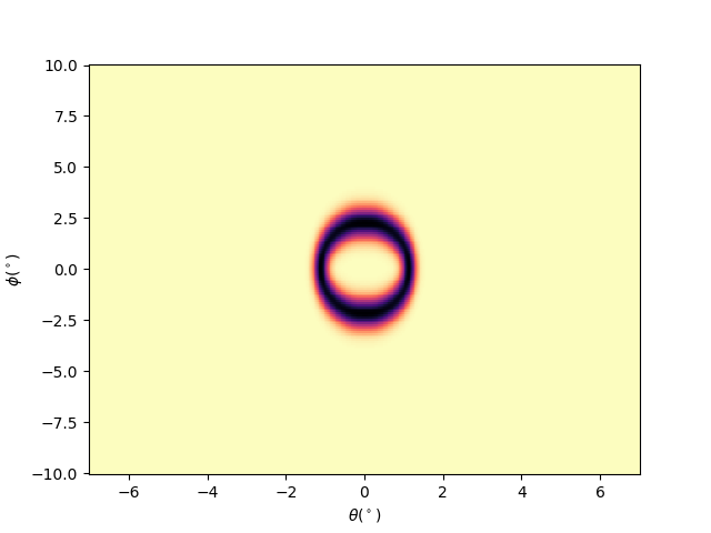
<matplotlib.collections.QuadMesh object at 0x7f6262db6a10>